Nov. 30, 2022

Coordinate frames and you

, , , , Leave a comment

It’s been a year since we last spoke. I thought that there couldn’t be a better topic to discuss than coordinate frames and rigid body transforms. </sarcasm>. In all seriousness, it’s a great concept to grasp solidly and hopefully will help you do the things that you do with inertial sensors more betterer.

Coordinate frames give you a reference of how you are moving through space. For a quick refresher, we understand that acceleration can be integrated to produce velocity, and velocity can be integrated to produce a relative position. This is all well and good, but if you do not have a proper understanding of which axis is forward, which axis is left, or which axis is up, integration of any of these data products will be wholly irrelevant.

Coordinate frames (based on our current understanding of the physical universe) are represented by three axis’, an X Y and Z. All of these axis are orthogonal to one another (simply meaning that they meet each other at 90 opposing degree angles). It can be somewhat difficult to understand which axis is which without a physical reference (a 3D object that can represent a coordinate frame that you can manipulate) or identification (a 2D image of a coordinate frame) to look at.

UNTIL NOW

…well, hopefully

Sidenote_00: I touched on this hand gesture in the last blog post, but it’s useful to go over again.

A useful thing to understand about coordinate frames is that most (used in evaluation of vehicle dynamics) follow a “right hand rule” convention. If you follow these steps below, you too can be like many physics / robotics researchers and make strange hand gestures when trying to intuitively comprehend coordinate frame rotations (which we will get to later).

– Make a fist with your right hand

– Stick your thumb out while still keeping the rest of your fingers in a fist

– Rotate your hand so that your thumb is pointing toward the sky

– Stick your pointer finger out so that it is pointing away from your body

– Stick your middle finger to your left

You have just created a coordinate frame. Following the right hand rule convention, your pointer finger is pointing forward and represents the +X axis, your middle finger is pointing toward the left and represents the +Y axis, and your thumb is pointing up and represents the +Z axis. You can represent any rotation of a right hand rule coordinate frame!

So now you’re probably thinking, “wow sander amazing”. I know. Just wait.

FLU, FRD, WAT?

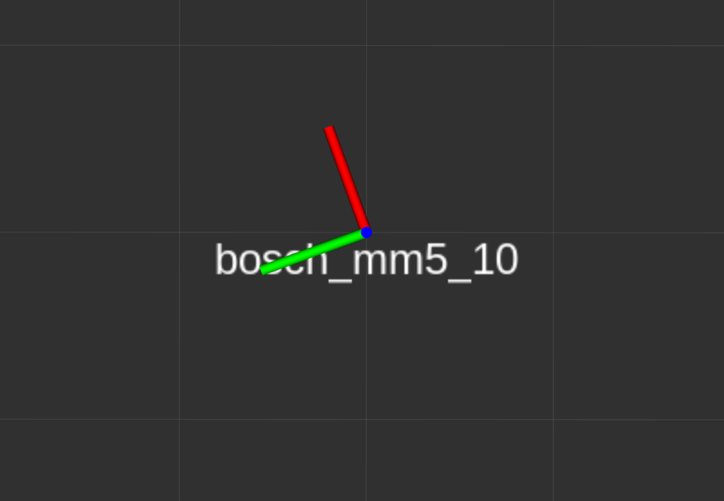
The Bosch Motorsport MM5.10 IMU is relatively ubiquitous and used in many race cars. A non-motorsport version is even shipped as standard equipment in some of the most popular electric cars that are on the public roads today. The MM5.10 sensor coordinate frame is represented by the same funny hand gesture that I just made you do. This is referred to in short hand as a FLU (Forward, Left, Up) frame. Meaning that X+ is Forward, Y+ is Left, and Z+ is Up.

Sidenote_01: This FLU frame is described by the ISO 8855 standard. Mainly used in ground traveling vehicles.

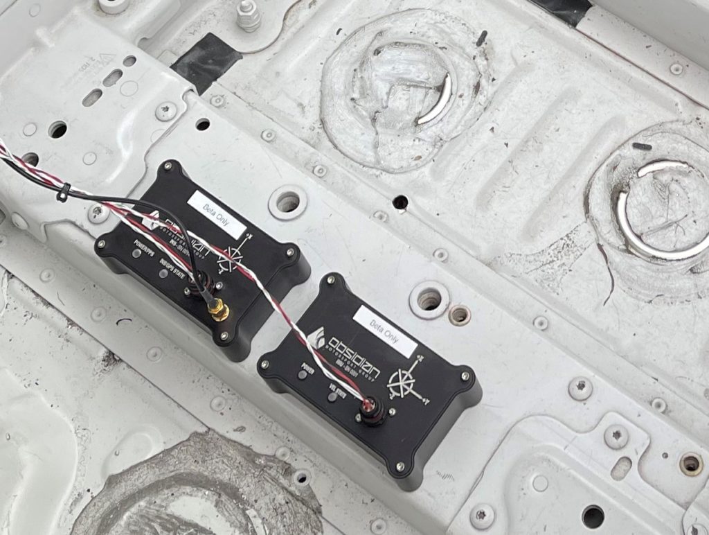
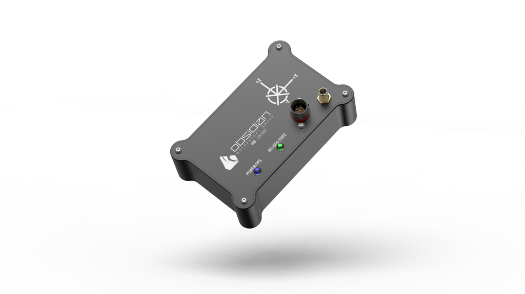
The Obsidian INS and IMU products use a different coordinate frame from the MM5.10 IMU. We use a FRD (Forward, Right, Down) frame. Meaning that X+ is Forward, Y+ is Right and Z+ is Down.

Sidenote_02: This FRD frame is described by the ISO 1151 standard. Mainly used in aircraft.

You’re still holding your hand in the hand gesture that I asked you to just a little bit ago, right? If that’s the case, you can easily rotate your hand around the X axis (your pointer finger, in this case) 180 degrees, and voila, you went from holding your hand originally in an FLU frame and now you’re holding your hand in an FRD frame. Using this hand motion, it’s relatively easy to come up with the intuition that, if we want to compare data between an MM5.10 and an INS we will either need to mount the MM5.10 upside down, or mathematically rotate it after the fact.

SIdenote_03: WAT

Aligning frames unrealistically

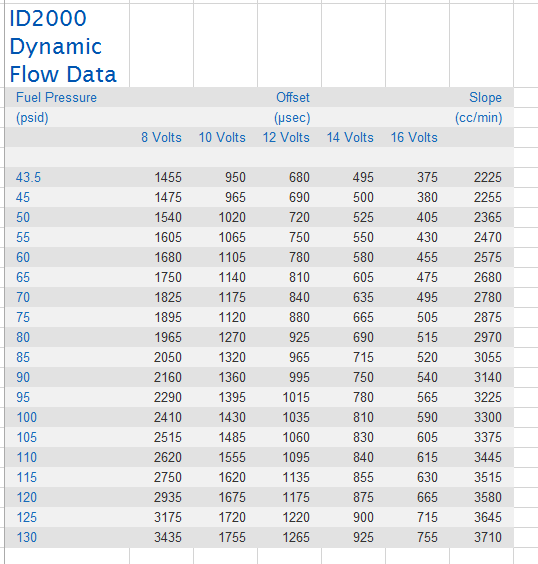
In practice, it’s normal to see a vehicle outfitted with one or more inertial measurement sensors and sometimes they can be from different manufacturers that have different coordinate frame standards. Using the examples above, lets assume for a moment that we have a vehicle with an MM5.10 using a FLU convention and an INS using a FRD convention. In this case we will assume that the MM5.10 is mounted directly on top of the INS (to reduce the math to pure rotation only).

Sidenote_04: Three color coordinate frames are usually represented by X == red, Y == green, Z == blue

MM5.10 IMU in FLU frame mounted above Obsidian INS with FRD frame

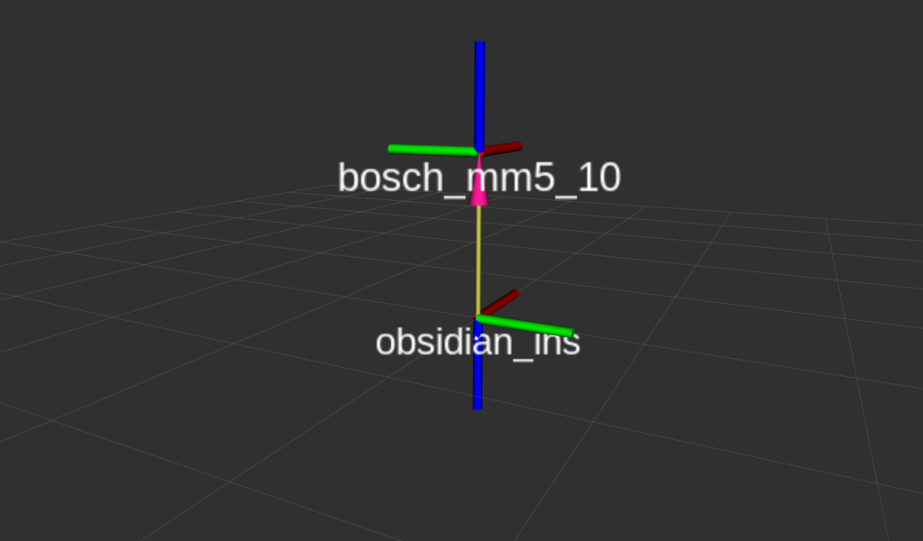
The dumb (and / or) simple way to align these two reference frames is to take the data products (accel and angular velocity) of the MM5.10 in the Y and Z axis and multiply them by -1. This will very simply invert the data produced from the MM5.10 on those axis’ and you will have successfully “rotated” the FLU frame so that is now an FRD frame. For example, you can take the Y axis acceleration of the MM5.10 and multiply by -1 and that acceleration will line up with the raw Y axis acceleration of the INS.

The visualized frame would mathematically look like this below:

MM5.10 IMU rotated from FLU to FRD coordinate frame, mounted above Obsidian INS. Notice how the axes are now aligned.

After rotation the MM5.10 in to the same coordinate frame as the INS, the angular velocities (yaw rate, pitch rate, roll rate) would theoretically be the same, and the acceleration measurements would be almost the same (we’re not accounting for translations here to keep this post a little shorter). Easy peasy.

Which way is positive?

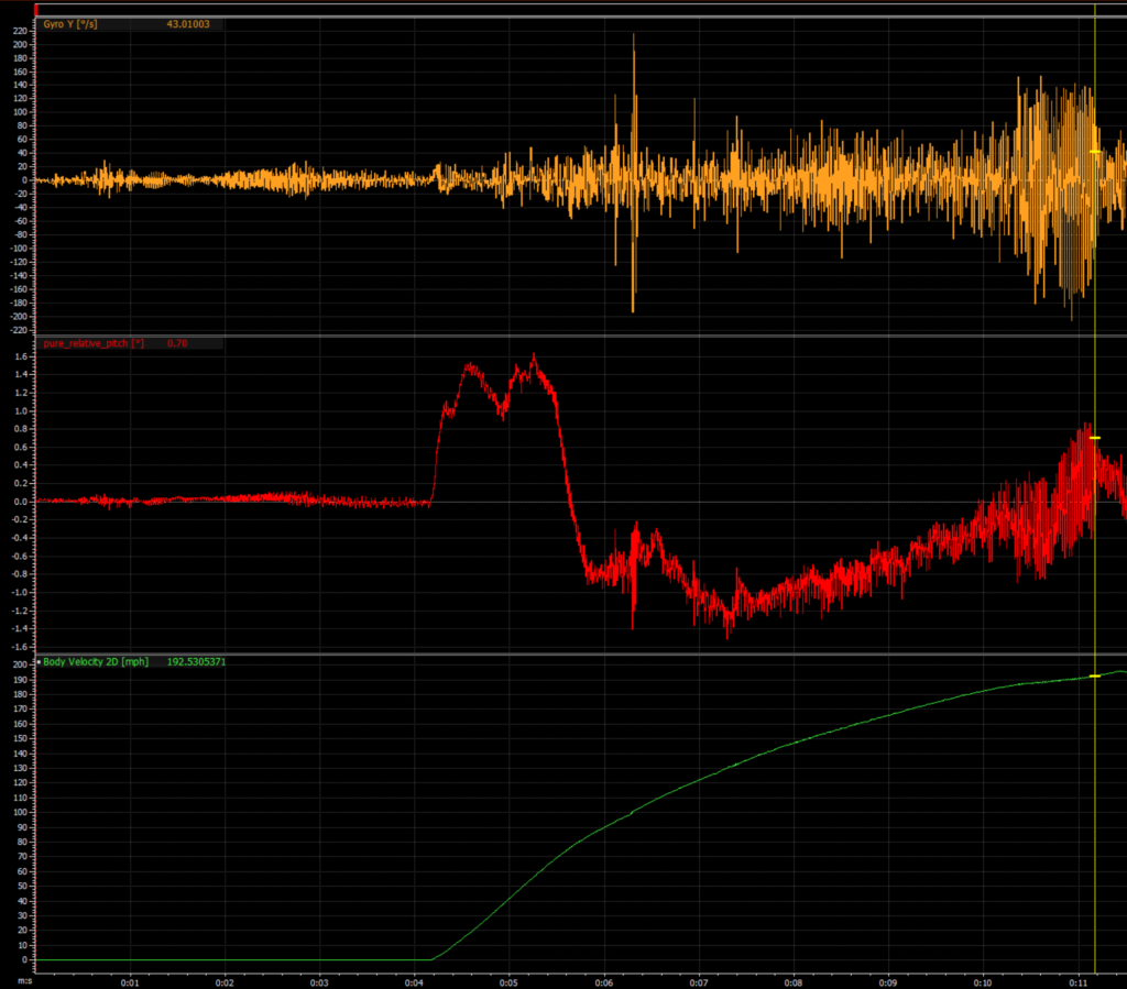
One of the most common questions I get about the INS / IMU has to do with direction of rotation. e.g. “Which direction is +10 degrees of pitch? Is the car pointing toward the sky or towards the ground?”. Thankfully, this is a fairly easy thing to intuitively solve when you use your very useful hand gesture that I described above.

Using your hand gesture, make a FLU coordinate frame to represent the MM5.10. This should make it such that your thumb is pointing toward the sky, your pointer finger is pointing forward, and your middle finger is pointing toward the left.

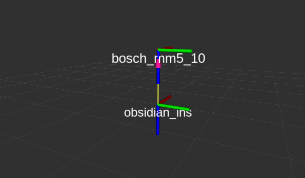
Maintaining that gesture, look at the tip of your thumb. If you rotate your hand around your thumb in a counterclockwise direction, this will be a positive rotation. The images below show a coordinate frame with a yaw value of 0, and a yaw value of +20 degrees.

A top down view of the MM5.10, looking in to the Z axis, where the X and Y axis are aligned with the grid below. This would represent a yaw value of 0.

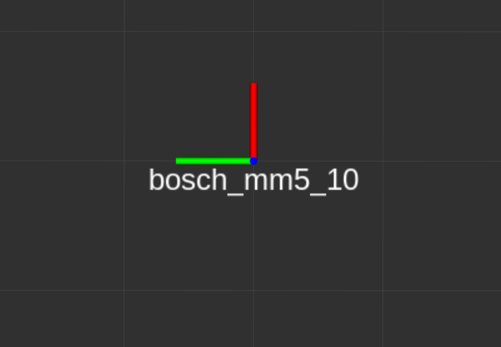
A top down view of the MM5.10, looking in to the Z axis, where the X and Y axis are rotated with respect to the grid below. This would represent a yaw value of +20 degrees.

The same thing would apply for pitch and roll, as well. “Look” in to the positive axis (In an FLU / FRD frame, X for roll, and Y for pitch), and what ever direction is counterclockwise will be a positive rotation.

Aligning frames realistically

While I’d like to tell you that you can align coordinate frames by multiplying with -1, that’s not realistic. We exist in a very non binary world. Which is great for everyone. Imagine how hard it must be for computers that only know 1 and 0.

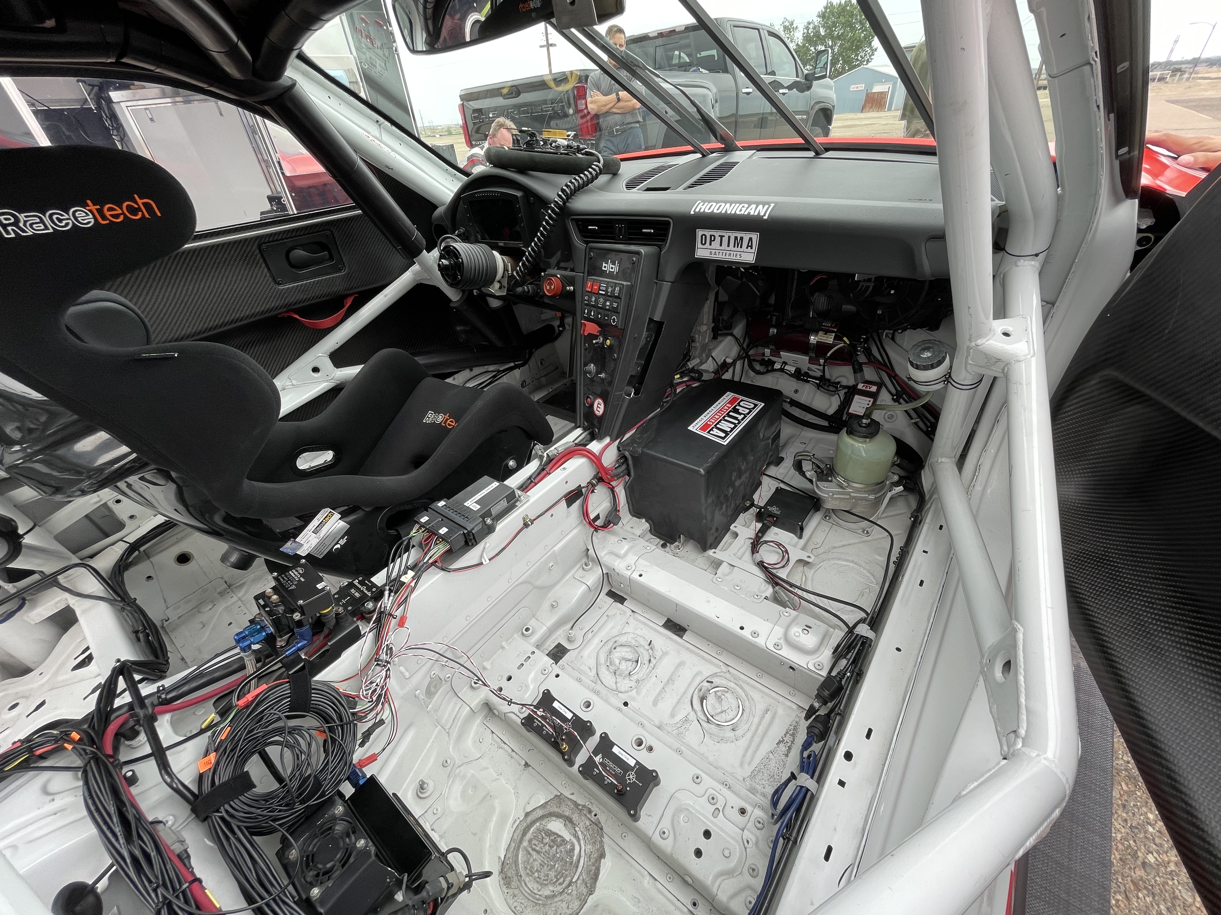
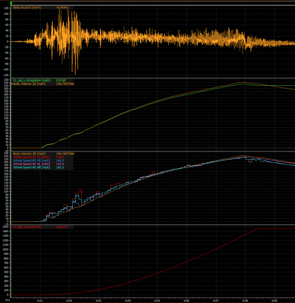
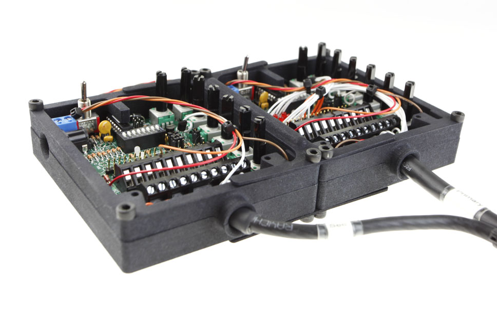
It’s not unrealistic to say that many race cars have less than perfect mounting of inertial sensors. In this example, let’s imagine a team trying to use an accelerometer in a dash logging display (MoTeC C1XX), or ECU (MoTeC M1XX) for driver analysis. It’s somewhat unlikely that the dash or ECU will be mounted so that the axes of the accelerometer are pointed exactly in the direction of motion that you are interested in (the vehicle’s natural coordinate frame). Maybe the dash / ECU is mounted “mostly straight” in the direction of travel, and / or “mostly perpendicular to gravity”. That doesn’t help us much if we’re trying to use this acceleration data for driver analysis.

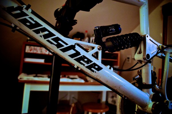
Imagine that we are trying to use a MoTeC C127 dash that is angled at the driver like this:

Borrowed from Google image search via a Rennlist thread.

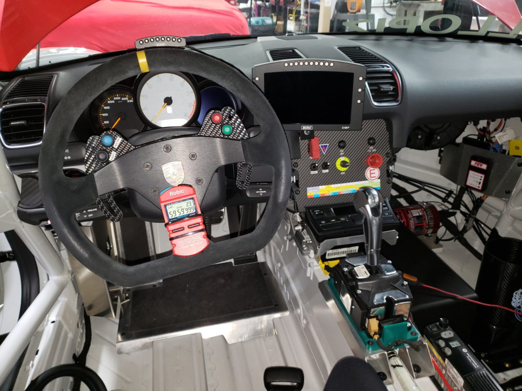
The MoTeC dash pictured above is angled such that the screen is visible to the driver. Being that the accelerometer in the MoTeC dash display is mounted to the PCB internal to the display itself, it’s reasonable to assume that the display being mounted at an angle will result in the accelerometer being mounted at an angle as well. In the interest of simplicity (as this post is already really long and we haven’t even done any math yet) we will assume that the MoTeC dash has zero roll, and zero pitch, with respect to the vehicle coordinate frame. The only thing we would notice in this case is that if the car is traveling exactly straight you may have acceleration in X and Y axes (assuming an FLU frame for the MoTeC dash itself and FLU for the vehicle frame).

MoTeC dash mounted with a -20 degree yaw angle with respect to the vehicle frame.

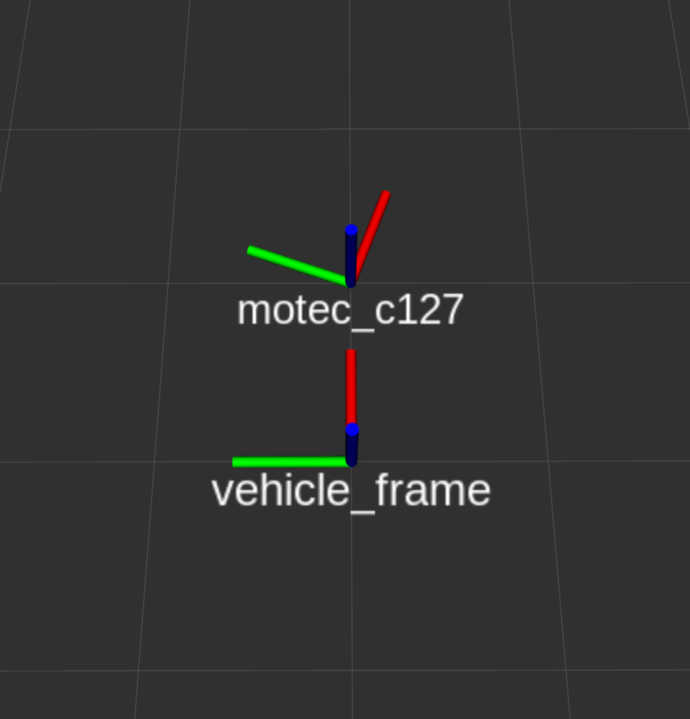
It’s relatively intuitive to see that if the vehicle is traveling exactly straight about the X axis (red in vehicle_frame), you will see acceleration in the X and Y axis in the MoTeC dash due to it’s mounting. Let’s work out how to mathematically rotate the accelerometer so that the data from the MoTeC dash is producing data as if it were mounted exactly straight (inline with the vehicle_frame).

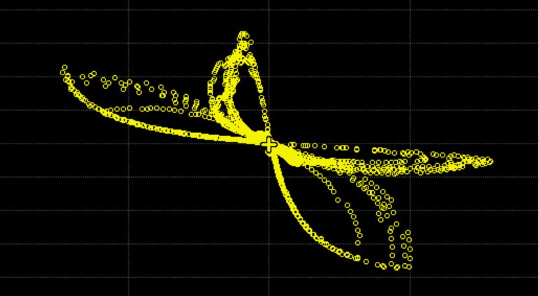
I’ve made some simulated accelerometer data from a MoTeC dash if the vehicle was traveling straight at 9.81 m/s/s constant for 1 second (sampled at 10khz), mounted at some unknown yaw angle with respect to the vehicle_frame above.

X, and Y acceleration in units of m/s/s (reminder 1G is equal to 9.81 m/s/s). X is in blue and Y is in orange.

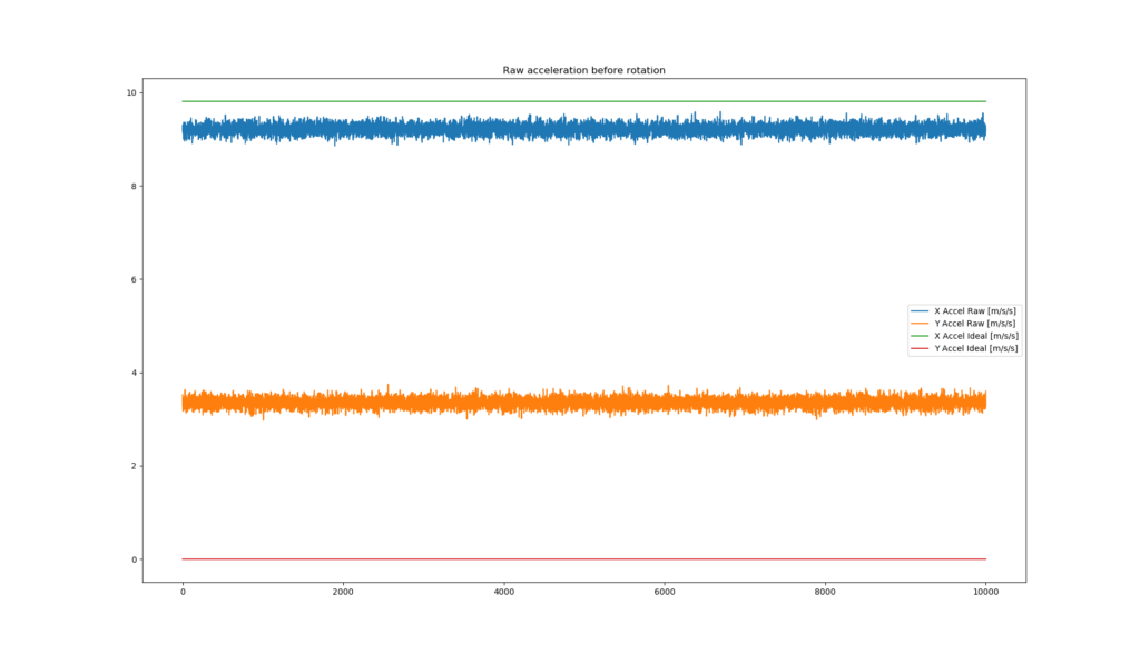
We can use the following steps to rotate this data such that it aligns so that Y and Z are equal to roughly 0.0, while X is equal to 9.81 m/s/s.

codenote_00: python-pseudo-code

# step 1
# find the mean of each axis of acceleration
ax_mean = mean(raw_accel_x)
ay_mean = mean(raw_accel_y)

# step 2
# "guess" a suitable yaw angle of the motec_c127 with respect to the  vehicle_frame
guess_yaw_degree = -15.0

# step 3
# convert guess_yaw_degree to radians
guess_yaw_radians = guess_yaw_degree * pi / 180.0

# step 4
# find the resulting acceleration after rotation using 1D rotation formula
corrected_accel_x = ax_mean * cos(guess_yaw_radians) - ay_mean * sin(guess_yaw_radians)
corrected_accel_y = ax_mean * sin(guess_yaw_radians) + ay_mean * cos(guess_yaw_radians)

# step 5
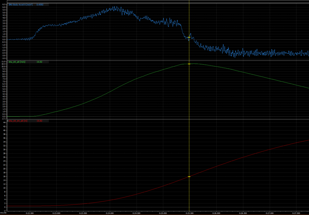
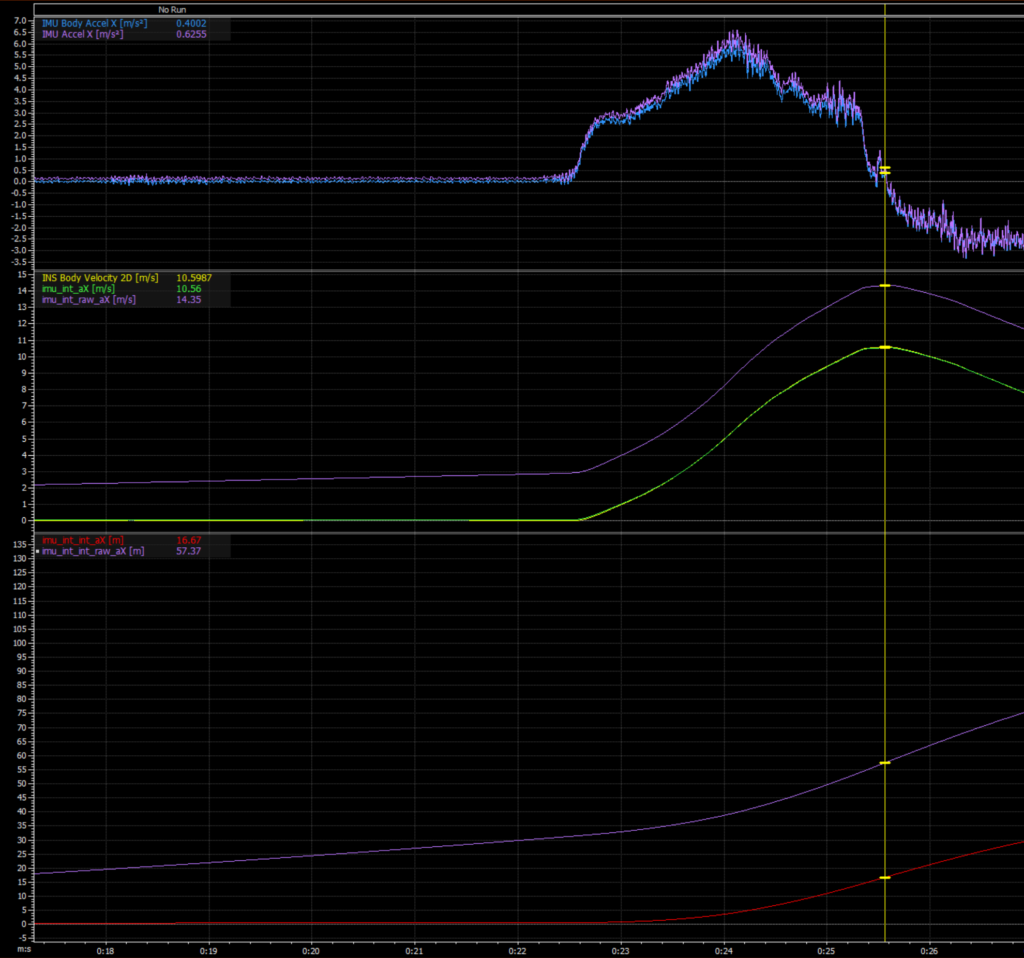
# repeat steps 2 -> 5 until your corrected_accel_x is equal to roughly 9.81 and corrected_accel_y is equal to roughly 0.0 

After you find your guess_yaw_radians channel, you can apply step 4 to all of your raw data and you should have a plot of data that looks like this!

You can see here the X and Y acceleration after rotation. The X accel is roughly equal to 9.81 m/s/s and the Y accel is roughly equal to 0.0 m/s/s

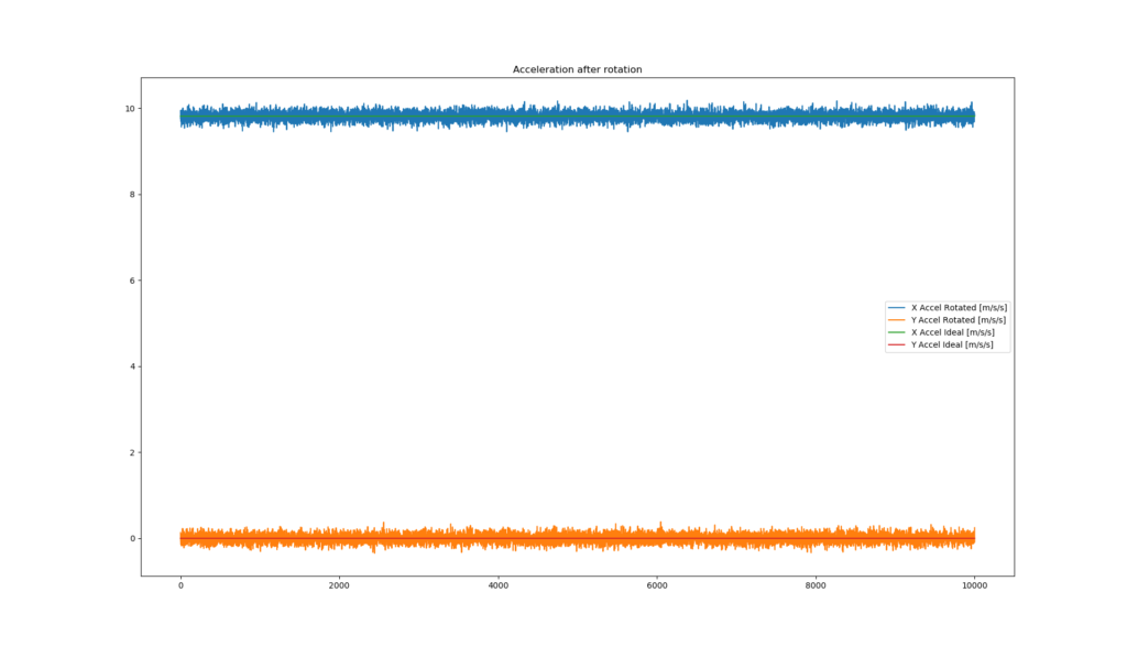
So, you’ve done it. After that work you should have successfully applied a 1D rotation to acceleration data and after this equation, the data from your MoTeC dash should have been mathematically corrected such that the data would be the same if the MoTeC dash were mounted in the same orientation as the vehicle_frame.

BUT WAIT. THERE’S MORE.

Imagine that the MoTeC dash needs to be rotated in more than one axis (yaw only in the example above), what about a yaw rotation and a pitch rotation? Or worse, what about a yaw rotation, a pitch rotation, AND a roll rotation? What are we to do?

The answer is much more complicated and much more difficult to hand estimate using a “brute force” approach that I’ve described above. It is made simpler by applying the rotation in one operation using a rotation matrix as opposed to euler angles* (roll, pitch, yaw), which can be very annoying to deal with when doing 3D rotations.

Sidenote_05: Euler angles are actually often misrepresented as Tait-Bryan angles.

Fin

I do realize that I glossed over details of translation components in proper rigid body transforms. Honestly, I didn’t realize that it would be this difficult to convey this concept in a pseudo-math pseudo-code way that was easily digestible while still keeping with my normal style of posts. Thanks for sticking with it. If you made it this far, you’ve earned some relaxation

Aug. 03, 2021

INS or IMU? It depends.

, , , Leave a comment

It depends how long it takes you to do what ever you’re trying to do.

There. That’s the end of the article.

Just kidding.

A Terminology Tangent

First, you’re probably thinking, “Tangent? This guy hasn’t even started writing anything yet“.

Second, I probably should apologize for having two products, that look nearly identical, that have nearly the same name, targeted at different applications, and with wildly different price tags. I am trying to take the Ron Swanson approach to making products. I’d like to just call things what they are. No marketing, no flair, no sponsored product placements. So, anyway, let me take a second and remind you, my loyal readership, what these acronyms stand for:

INS stands for Inertial Navigation System. This is an industry term in robotics that, generally speaking, defines a system that is a GNSS receiver, accelerometer, gyroscope, barometer, and temperature sensor (among other sensors, sometimes) combined together with a complex sensor fusion algorithm to produce a single high-rate, high-accuracy 6DOF pose (and corresponding derivatives that we will talk about later in this post).

sidenote_1: 6DOF Pose stands for 6 Degree Of Freedom Pose. These 6 individual degrees of freedom are: Roll, Pitch, Yaw, X Position, Y Position, Z Position. When combined, they represent the position of the sensor in a 3D world.

IMU stands for Inertial Measurement Unit. This term is a bit more complicated. This is also an industry term (in robotics, and motorsport at the sub-pro level) that, generally speaking, defines way way too many different sensors, systems, and products.

In motorsport, an IMU is generally defined as a sensor that will give you acceleration, and angular velocity. It is generally a very basic raw sensor output with no sensor fusion or on-board math going on.

In robotics, an IMU is generally defined as an accelerometer, gyroscope, barometer, and temperature sensor combined together with a complex sensor fusion algorithm to produce high-rate / high-accuracy orientation (roll, pitch, yaw), acceleration, and angular velocity.

INS on the left, IMU on the right
The PPIHC Open Class champion that I was able to use as a test platform to benchmark some new INS and IMU beta features

So, as you can probably tell at this point, I’m following the terminology of the robotics world in naming these two products. The robotics definition of the INS is what the Obsidian Motorsport Group INS is. The same is true for the Obsidian Motorsport Group IMU.

Derivatives and Antiderivatives

I know, scary math word, but please relax. I’m going to do everything in my power to use intuitive examples to demonstrate some things about how the IMU (and to some extent, at a very basic level, the INS) derive some of their more interesting data products.

Derivatives are simply the representation of the change of something divided by the time it took to make that change. Antiderivatives (also referred to as Integration) are the opposite. Stay with me here, practical examples that are not your run of the mill “passenger on a train” physics examples are incoming…

Lets assume that you have a general purpose 3-axis accelerometer mounted in a vehicle, rigidly attached to the chassis, and the X-axis is pointed forward, the Y-axis is pointed left, and the Z-axis is pointed up.

sidenote_02: This accelerometer mounting mentioned above (and our INS / IMU…) follows a “Right-Hand Rule” convention. If you curl your right hand in to a fist and rotate it such that your thumb is up, and do the following:

  • Point your pointer finger forward
  • Point your middle finger toward the left
  • Point your thumb in the air

Your pointer finger will be the X-axis, your middle finger will be the Y-axis, and your thumb will be the Z-axis. No matter how you mount a “Right-Hand Rule” IMU, if you keep the finger-to-axis assignments the same, you’ll be able to envision what the coordinate frame looks like with your hand! Neat.

Using the coordinate reference frame mentioned above, when the vehicle travels forward, there will be positive acceleration present in the X-axis.

  • If you integrate the acceleration (using units of m/s/s) in the X-axis, you will get velocity (using units m/s) in the X-axis.
  • If you integrate the velocity (using units of m/s) in the X-axis, you will get position (using units of m) in the X-axis.

The picture below should illustrate that point well.

  • The blue trace at the top is a measure of longitudinal acceleration (forward + / backward – ) in units of m/s/s.
  • The green trace is a measure of longitudinal velocity in units of m/s. This is a result of integration of the blue trace.
  • The red trace is a measure of longitudinal position in units of m. This is a result of integration of the green trace.
Acceleration (top), Velocity (middle), Position (lower)

sidenote_04: It’s important to remember that there are a lot of factors that go in to creating an accurate acceleration measurement to do these integrations off of. You should absolutely try this on your own with whatever sensor you want to use, but be warned, It’s harder than you think to do this with a basic accelerometer.

So, now you know the relationship of acceleration, velocity, and position. I feel pretty strongly that this is an important concept to grasp to discuss the next part of this post…

Error

Now that we know how integration works, intuitively anyway, we can talk about the biggest issue with integration: error.

Accelerometers are not perfect instruments. Even the fanciest ones on the planet are prone to small error based on a multitude of factors (Namely temperature for the ones that normal civilians have access to). When we integrate acceleration to get velocity, any small error in acceleration, will propagate forward as an error in velocity. This is compounded when we integrate velocity to get position!

The picture below, should illustrate that point well. It is the same data as the trace above, but with some error introduced in the longitudinal acceleration measurement. Check out the position error at the end, it’s ~40m !

  • The purple trace at the top is “nearly” the same acceleration as the IMU Body Accel X [m/s/s] channel.
  • The purple trace in the middle is a result of integration of the purple acceleration measurement at the top. Notice the significant error (~4 m/s).
  • The purple trace at the bottom is a result of integration of the purple velocity trace in the middle. Notice the massive error (~40m).
The two acceleration channels don’t look that different, do they…

Our IMU goes through a factory calibration at the chip level, then a second calibration (at our office) to try to do our best to remove any errors that are introduced after installation (soldering). We spend a lot of time with this to try to give you acceleration data that is in blue, and not in purple.

In addition to our calibration processes, there are online algorithms that are running that are constantly (on the sensor itself) trying to estimate and correct any errors in the acceleration and gyroscope measurements to make sure that we’re providing you the best data possible. However, since those algorithms have no real understanding about how the vehicle is moving through the world (say, with a GNSS / GPS receiver like the INS…), these bias correction algorithms are only effective to a point. This “point” is about 30-45 seconds after the vehicle has left the starting line and the integration process has begun.

Do I need an INS or can I use an IMU? TELL ME, SANDER.

Okay, okay. I hear you.

The IMU is explicitly designed for standing start, ground vehicle, racing that lasts for less than 30-45 seconds.

The INS is explicitly designed for everything. Since the sensor has a GNSS / GPS receiver on board, the sensor can automatically mitigate biases that creep in over time to the accelerometer and gyroscope. It has no time bound.

The IMU will provide the following data products at up to 800hz:

  • Ground Speed*
  • Raw Acceleration (X, Y, Z)
  • Body Frame Acceleration (X, Y, Z)
  • Angular Velocity (X, Y, Z)
  • Orientation (Roll, Pitch, Yaw)

*The IMU will need to be sent a simple CAN message to tell it that the pass has started to generate Ground Speed. It’s easy to do, I promise.

The IMU will have the following features:

  • Adjustable baud rate (1mbps default, 500kbps, 250kbps)
  • Adjustable transmission rate (800hz, 400hz, 200hz, 100hz, 50hz, 25hz, 10hz).
  • Adjustable user tunable filters for acceleration / gyroscope data
  • Advanced Kalman filter tuning parameters

The sensor will be sold for $1750 and I will have a number in hand to sell in about 3-4 weeks. As always, if you have any questions, please email me at sander 4T obsidianeng d0t com

Now, you may be thinking, “Sander, you could have lead with that and I wouldn’t have had to read this stuff about derivatives, integration, and error propagation.”

You’re right. I could have.

Dec. 23, 2020

GPS? IMU? INS? What on Earth even is that?

, , Leave a comment

See what I did there?

I should start out by saying it’s been quite a while since I’ve written anything in a “blog” type format, so please be patient if I go off on a long tangent about something that’s powerfully uninteresting to you, my loyal readership.

Since my last post on this blog, I moved to California (San Francisco, specifically), got hit by yet another car while riding my bike, ate many delicious meals in San Francisco, had many successes with work, learned many hard lessons about living in a city, learned many more hard lessons about working with OE manufacturers on engineering projects, and (more relevant to this post) using / understanding / configuring / and making sense of Inertial GPS systems. Let’s go over some basics about the latter.

GPS / GNSS:

Many moons ago, I thought that when you placed a GNSS receiver / antenna on the roof of a race car, you could power it on, science would happen, and then it would tell you where on the earth you were. Magic.

I didn’t spend much time thinking about how it worked, because, well, it worked fine. It provided a nice visualization of where a car was on track. Fine. Great.

Over the past few years it has become increasingly obvious that it’s really important to understand how something works if you’re going to rely on the data it produces. A lot of the projects that I have been involved with over the past few years at some point rely on GNSS. It’s really important to know when to rely on it, when not to rely on it, and why.

sidenote_1: Sander, you keep writing “GNSS”, what does that even mean? “GNSS” stands for Global Navigation Satellite System. Some people often say “GPS” when they actually mean “GNSS”. You could plausibly argue that GNSS and GPS are interchangeable as ways to describe a system that can calculate where you are on the earth, but I felt it was worth mentioning that. GPS is actually a constellation (series of satellites in a specific orbit around the earth) of satellites that are owned and operated by the US Space Force. Yes, that Space Force. There are other constellations that are run by other countries such as “Galileo” (EU), “Beidou” (CN), “Glonass” (RU), “IRNSS” (India), “QZSS” (Japan). A GNSS system may use signals from satellites from one or more of these constellations to calculate your position on the globe. Neat right?

So, this begs the question: How do GNSS systems determine your position? How does it work? SANDER, TELL ME HOW SCIENCE HAPPENS!

sidenote_2: I’m going to do a super high level description of how things work, but if you’re interested in much more detail, you should really checkout this GPS Compendium (by u-Blox AG). It is a treasure trove of information about GNSS systems.

Basic things to know:

  • There are a number of satellites (in different constellations, run by different countries) orbiting the earth in a known trajectory / orbit.
  • Each satellite has an atomic clock on board to keep accurate time.
  • Atomic clocks are cool because they keep very accurate time for a very long time. (Not like your calculator wrist watch that you’re wearing right now. yes, you.)
  • Satellites regularly transmit their time so that GNSS receivers on the ground can receive this information.
  • If you take in a known position of the satellite, time from the satellite, you can use the speed of light as a constant to determine the distance from the GNSS receiver to the satellite.
  • You can determine a 3D position and time error with a minimum of 4 satellites. (Latitude, Longitude, Altitude, delta T error).
  • There are many sources of error that can cause accuracy issues (ionosphere time delay, multi-path signal errors, and other things outside the scope of this post)
  • The rate in which data is sent from these satellites will limit the rate at which we can calculate our position on the ground

That last bullet point is really the key issue here. Even very very expensive GNSS systems (NovAtel et. others) can not generate high frequency position measurements (lots of position updates every second) with just GNSS data alone. You need more data to help “fill in the gaps” between GNSS position updates. Well, how on earth would we “fill in the gaps”???

IMU (Inertial Measurement Unit):

IMU’s are generally understood to consist of a 3-axis accelerometer and a 3-axis gyroscope. What even is that? Let’s start with the accelerometer.

IMU (Accelerometer):

Like the name implies, the accelerometer measures acceleration. Now, you may be thinking, “Wow, Sander, you’re blowing my mind right now”. Or, maybe you’re not thinking that, hard to say.

I know that’s inherently obvious based on the name, but another way to think about acceleration measurement is that there is always acceleration to be measured (at least on our planet) by way of gravity. If you set a 3-axis accelerometer on a flat table, you will notice that the axis that is pointing up will report approximately 9.81 meters / second / second of “acceleration”. This is the measurement of gravity acting upon the table to keep it from floating away.

What can we do with an accelerometer beyond all of the well meaning, but painfully over simplified, statements about “my car pulled 3g’s off the line” or “I saw 2.5 lat G in T5 at Summit Point”? We can use calculus! From acceleration we can determine velocity doing a single integration, and we can determine relative position doing a double integration!

sidenote_3: I’m intentionally skipping an entire large chunk of explanation about removing gravity from acceleration measurements to actually get something useful from them and before integration to achieve velocity measurements, and entirely skipping bias calculation / error sources, for now.

This example shows live data from our INS (Body Accel X [m/s/s] and Body Velocity 2D [mph]). It also shows that you can integrate the Body Accel X [m/s/s] data and return velocity in the X axis ( t1_vel_x_integration [mph] ), and even distance traveled ( t1_dist_traveled [ft] )!

sidenote_4: Live distance traveled channels are being prototyped now and will be added to the sensor firmware later in 2021.

IMU (Gyroscope):

Like the name implies, the gyroscope measures gyroation. (Sorry, this is wildly incorrect, I just thought it would be funny at the time of writing relative to my previous bit about accelerometers measuring acceleration).

Gyroscopes measure the angular velocity about an axis. A simple way to think about this is if you placed a gyroscope on your hipster friends turntable (ya know, for vinyl records), and turned it on, the axis that is pointing straight up will probably indicate ~200 deg/second (33.3 RPM for 12″ records). This is simply measuring the speed at which the turntable is spinning.

What can we do with a gyroscope beyond making your friend with the turntable nervous by telling him it’s actually spinning at 198 deg/second as opposed to the 199.7999999999999999 deg/second it should be? You guessed it, more calculus! From angular rate we can determine the relative angles (more simply put, relative roll, pitch, and yaw) doing a single integration!

sidenote_5: It’s important to remember that in a rigid body (something that doesn’t flex or distort about the axis in which you’re measuring), the angular velocity (and resulting angle after integration) will be the same no matter where you place the gyroscope on the rigid body. Another way to think about this is simply that if you have a motorcycle that does a wheelie, no matter where you mount a gyroscope, the resulting pitch angle after integrating the pitch rate will be the same. 

This example shows live data from our INS on all channels.

sidenote_6: The pure_relative_pitch [deg] channel has a simple subtraction function to compensate for the mounting of the sensor in the vehicle. The live pitch measurement from the sensor will be absolute pitch (relative to gravity vector).

IMU (Error):

IMU’s are great because they can be light and small and provide very high rate data (1khz +), but it is also important to remember that they can be subject to long term integration error. These errors are omnipresent in in all IMU’s but especially ones that us common folk (read: not military) are allowed to buy.

Cheap IMU’s (less than a $10,000.00 or so) are usually Micro Electrical Mechanical System (MEMS) based units. They’re great because they’re small, cheap, light weight, and low power. But they are prone to massive error (usually mainly based around temperature, but there are other sources of error, too) if doing numerical integration over long time windows.

sidenote_7: “…long time windows” are definitely relative. Many consumer grade sensors (cheap) can even start showing integration error in seconds! On the flip side, many tactical grade (usually military only and > $10,000) will measure their integration error in hours)

These errors are tough to calibrate out, and are better addressed if you have another reference to compare your velocity and position to, periodically.

INS (Inertial Navigation System):

Here are some things we now understand:

  • GNSS systems can be highly accurate, but the rate at which they can provide position updates is relatively slow.
  • IMU’s can provide very fast measurements from which you can determine position, velocity, and orientation. However, their accuracy can become quite poor very quickly when doing single (or double) integrations.

An Inertial Navigation System (INS), combines these two sensors and uses the global accuracy of a GNSS system and the speed of an IMU! These INS systems use some derivative of a Kalman Filter (non-linear Extended or Unscented) to combine these sensor inputs perform what is sometimes called “Sensor Fusion” to generate one smooth cohesive output.

sidenote_8: Kalman Filters are a constant source of interest and wonder, however I think explaining how they work is outside of the scope of this blog post.

What is the point of this wall of text:

Well, I have put together an Inertial GPS system that I would like to sell. I am simply calling an INS. It uses a tried and true Extended Kalman Filter that is very robust and platform (or motion model) agnostic (car, motorcycle, plane, rally-car (read: plane)). I have tried really hard to make integrating this sensor as easy as is humanly possible to any modern, high-end data analysis / control system.

Here are the features:

  • 400Hz 32-bit Position (Latitude, Longitude, Altitude)
  • 400Hz 32-bit Velocity (Body X, Body Y, Body Z, and 2D Speed)
  • 400Hz 32-bit Body Frame Acceleration (Gravity Removed) (X, Y, Z) with online acceleration bias compensation
  • 400Hz 32-bit Angular Rate (X, Y, Z) with online gyro bias compensation
  • 400Hz 16-bit Orientation (Roll, Pitch, Yaw (Degrees))
  • 100Hz “MoTeC GPS” simulation option for integration with MoTeC M1 ECU applications with locked firmware (GT-R, Lamborghini, etc…)
  • CAN (1mbps) Output
  • Extensive integration support (MoTeC Dash Config, MoTeC M1 Build Project Module, DBC file)
  • CNC aluminum enclosure with Deutsch ASL connection and optional IP68 sealing
  • Custom firmware available for customer specific addressing, precision, transmit rates, conversions, units, additional on-board math channels, etc…

On the www.obsidianeng.com/downloads page you will find manuals, DBC files, MoTeC dash configuration files, and MoTeC M1 Build Modules.

The sensors will be available for purchase in Q1 2021. The cost will be $4500.00. Please shoot me an email (sander at_sign obsidianeng.com) with more questions.

Feb. 25, 2017

sander, what are you doing?

, Leave a comment

I will tell you, but first, a story:

For those that may not know me very well, I’m a pretty avid cyclist and general two-wheeled user of things. My interest mainly lies in mountain bikes and most things involved with dirt, but occasionally I’ve been known to do the group road ride or two. A few years ago I was sweeping (at the back) a group ride of about 8-9 people near my house and toward the end of the ride, I was plowed in to (rear ended at around 35-40 mph) by a young driver. I was knocked out, and was banged up pretty bad. Split my helmet, too. Had I not been wearing it that night, I would almost surely be in a different position / state of life at this moment.

Sidenote: bike frame was good, though (for those wondering). Steel is real, man!

Since then, I’ve been admittedly timid about getting back out on the road, but I’m slowly getting my head around being back out and have done a number of really stellar road rides since then. One of the things I’ve noticed as I’ve ridden / driven around in the years since then is that people are paying less and less attention to the act of driving. Cell phones, our ever increasing need to be busy and productive during every second of our lives, and the arguably increasing number of gadgets in cars today are preventing a genuine focus of driving.

Now, if you’re thinking, Sander, WTF are you getting at here? I’ll wrap it up.

An opportunity appeared a few months ago to start doing some research work on the vehicle integration / control side of an autonomous vehicle. Honestly, I didn’t think about that whole bike thing when I initially agreed to the research work (I mainly just thought the mental food / challenge was completely awesome), but as I’ve come to understand the challenges (chewy, incredibly interesting challenges) and numerous potential advantages to autonomy it’s made me revisit that whole scenario. I am 100% confident that that incident could have been prevented with technology that’s currently in rapid development or even already available.

The point of this is that I’ve agreed to take a full time position at the company who hired me to do the research work a few months back (I’m intentionally holding the name of the company back until a later date).

Internal combustion control will always be my first professional love, but it feels pretty stellar to work on something that could actually aid in saving someone’s life.

Obsidian Motorsport Group will still be “open” but just in a very limited capacity.

If there are any questions, please email me directly from the contact page.

Thank you to all of my customers and friends who have helped me to get to this point. Truly.

scatter_snip

Nov. 16, 2015

you should really know what you’re doing

, , Leave a comment

you should really know what you’re doing.

11/16/2015

We’re not all born with knowledge. We’ve got to work for it.

I guess I could have entitled this post “really useful stuff you can do with a simulator”, but I think that the current title is equally effective.

A long while before this current moment, most of my pre Obsidian Motorsport Group professional life was based around figuring out problems. (I promise that I’ll try and keep the retrospective of my younger self to a minimum). I started my automotive life as a sophomore high school kid working at an automotive repair shop. They did general repair and specialized in fixing old air-cooled VW and Porsche engines. Looking back on that job, I think that it really gave me a solid foundation for my professional life (and arguably my personal life, too), but at the time that I was there, I hated it.

The reason for all of my misplaced adolescent hatred was based around the idea that my bosses (two guys) wouldn’t ever allow me to just replace a part to see if the problem got better. They required me to prove that every part I replaced, needed to be replaced. If that involved showing them there was a definitive dead short in a harness with an ohm meter, or showing a oscilloscope capture of an M112/113 Mercedes crankshaft position sensor as it loses its amplitude when the sensor gets hot. Again, hated it at the time, but it really beat in to my brain that it’s best to prove your hypothesis before jumping to a conclusion.

jump_to_conclusions_mat

(…I just had a great idea)

Fast forward to now, the mindset of proving your actions with quantitative data is really the basis of what I’m trying to demonstrate the power of.

Here are some basic examples of things that are made easier with a simulator:

4344_small

Do you know how the VE model works?

Fueling is (for me, anyway) one of the more interesting variables in an engine management system to wrap ones head around. As a basic recap, fuel injector pulse width is the output of an equation inside an ECU taking in to account a number of different sensor values. IPW is the amount of time that the ECU commands the injector to be open. The amount of fuel that is delivered from the injector during this on time is based on fuel pressure, measured injector flow rate, battery voltage, and density.

The following truth is unfortunate: You don’t need to know about any of that stuff (or the ideal gas law) to tune an engine mostly well with newer volumetric efficiency based ECU’s

You can pretty much input a few simple variables and set the VE table to 90 and the engine should start up and run mostly well.
So perhaps being ignorant of the ideal gas law or what determines injector on time, figure you’ve bumbled through the map enough to get the car running pretty solid and making a “number” for the customer. Great. Good for you. Say the customer comes back and wants you to install a flex fuel sensor and re-tune for E85 or E98 or something of the sort. Are you confident that the ECU is going to add the appropriate amount of fuel over your pump gas tune when you go to make that first dyno pull on E85? What about using multiple ignition tables? Do you know that the blend table is going to work correctly? What happens if your VE table is only scaled out to 20 psiG, and you have a run out to 25 psiG, what’s the ECU going to do if you ride off the end of the table?

That can all be simulated, on your desk while you’re sitting in your favorite thinking chair.

Beyond the initial benefit of just seeing what’s going to happen to the injector pulse if you add in some ethanol content or drive off the end of the load axis, you can spend the time to reverse engineer the fuel model that is being used in the ECU. I may be a bit of an outlier in this department, but I try not to trust or have faith in anything I don’t understand or haven’t tested, first.

What about fuel compensations / trims?

Not all ECU’s are created equal in this department. How do you know if the ECU uses a multiplier or a percentage value? You would think that this would be easy to find in some ECU software programs, but it is not always as easy as one would think. It’s a lot more relaxing to do that with a simulator and move independent values around to see how it is affected before you get to the dyno / track.
Are these the same? (Emtron and MoTeC)

(picture will be replaced, soon)

I should take a second here and give an honorable mention to Life Racing’s LifeCal. They have an awesome, easy to read layout of the entire fuel calculation. See picture below:

life_fuel_calc

What about secondary injection / blend tables?

Not all ECU’s are created the same here, either. Some of the wording is a little opaque on the Mx00 MoTeC ECU’s when it comes to secondary injection

What about boost control?

If you’re the type of guy or girl who just likes to “let it eat” with open loop wastegate duty cycle controls, then this probably doesn’t matter much to you.
However, if you take pride in what you do and find a need for precise boost control, getting a feeling for the PID sensitivity controls is much more relaxing at home with a cup of coffee or any other preferred beverage of choice. PID settings are ECU manufacturer specific. Settings that work in an AEM V2 / EMS4 box WILL NOT work in an MX00 MoTeC ECU and vice-versa.

What about traction control?

Yes. This is where simulators are pretty great. The MoTeC M800 ECU’s have awesome traction control settings. The power of the M800 is the ability to make tables and compensations acting on other tables or compensations. After you get through a few levels of that, it can get a bit heavy to wrap your head around. So if you are using one of the Intermediate or Advanced simulators, you can simulate a driven wheel speed to see what’s going to happen with the timing, drive by wire throttle, fueling, or limiters BEFORE you get to the track. If you take a second to think about all of the time that can save you, it’s pretty immense.

What about setting up CAN devices to talk to each other?

You CAN do that pretty easily (I know, I’m hilarious). CAN stuff isn’t bad to do if you’re using all MoTeC products, as they provide really easy to set up templates. However it CAN get a BIT (sorry, I’ll really stop now) more difficult if you’re using MoTeC dash loggers and an AEM ECU (or Cosworth ICD and a Bosch Motorsport ECU or any number of other combinations) If you wanted to utilize all of the CAN data sent over from the AEM ECU, you would have to write a custom can template. This is not too bad to do if you can simulate values (say RPM for instance) in to the AEM ECU, connect the MoTeC dash to the AEM ECU via CAN and then work on the scalars and multipliers until the value is correct in the MoTeC dash.

So, why did I start this post by talking about myself as a young all-knowing teenager? Because I used to think that it was stupid to have to prove your work. If I could get the car fixed by guessing and maybe getting lucky, then that was good enough. The truth is that it’s really not good enough. If you can get by moving numbers around and making some power and you’re ok with that, then great. Although, I think that what’s going to separate “tuners” from professionals is knowledge and understanding. Buying a simulator isn’t going to give you the knowledge and understanding, but it can help you gain it much easier and much more safely. (and, it’s entertaining if you’re easily entertained).

2015-02-10 18.50.05

May. 15, 2015

knowledge reigns supreme over nearly everybody

, , , Leave a comment

knowledge reigns supreme, over nearly everybody

5/5/2015

I have been spending way too much time recently thinking about how I can convey the importance of data systems to you, my loyal readership. It’s the most important tool a team has in making strides in performance, diagnosis, and reliability. That’s really the best thing I can come up with. It’s used in EVERY professional race series, regardless of category. If that’s not enough to sway you toward a data system, then I’ll continue to ramble about it below.

I am in an interesting position in that I do private label work for a number of shops, teams, and individual customers. Basically, I get to see a lot of different stuff. I’ve done data analysis for a NASCAR Sprint Cup team, I’ve done analysis work for club level road racers, snowmobiles, drag racers, and a whole load of high performance street cars. The thing that all of these groups and categories have in common is that they all require some type of way to review and analyze data. Engine mapping, troubleshooting, and performance are all quantified and adjusted based around data. This all sounds super great, right? It is. Super great. But, it seems that there is a disconnect when it comes time for my customers to purchase one of these systems. Here are two problems that I’ve noticed over time.

The perceived gain problem.

There is a big problem with the understanding behind purchasing data systems. The problem, as far as I see it, is that there’s no direct connection in a customer’s mind behind purchasing a data package and performance gained.

For instance, customer A wants to buy a turbocharger that has a 50lb/min max flow rating. His current turbo is 30lb/min. This will yield an approximate 200 hp gain (all things being fair and equal in the world of physics). Customer A will go to a dyno, get his engine mapped, and there will be a before and after chart representing the difference in power. He will see and feel the money that he spent. With 200 extra hp, maybe he’ll drop 2-3 seconds off his lap time. Maybe. That’s if the extra power doesn’t through the cars balance off, or over drive the tire, or over heat the brakes.

What happens if the customer is told that he can spend the same amount of money on a data system that could take 5.00 seconds off his lap time by using accelerometer data and driving line evaluation, potentially identify faulty sensors, potentially identifying an engine failure BEFORE it happens, and allow for peace of mind if all of the data looks great?

He’s going to go for the turbocharger.

The problem at hand is that there is no perceived direct correlation between data and performance. It’s unfortunate because, when used correctly, this couldn’t be further from the truth.

Now it’s probably obvious by reading the other content on my website that I sell data systems, and it would be great if you contacted me to talk about them in more detail. But, all bias aside, they really are useful pieces of equipment that sometimes can result in the dramatic lap time reduction mentioned above, among other useful purposes.

Thoughts on being emotionless.

There’s such a nice feeling associated with making decisions based off of objective data. It completely removes the need for “emotion” or “feelings”. In the context of engine mapping, this concept couldn’t be more true and to the point. Imagine you’re sitting in the drivers seat of a 1000 hp Supra strapped to the dyno and you’ve just started a pull in 4th gear. You’ve got a lot going through your mind. “Does this engine have a coolant leak?” “Does it actually have E85 in it, or is it diesel?” “What’s that sound? Rod knock? Valve tap? Oil spraying out of the cylinder head?” The list goes on and on. And then you’ve got the normal stuff you’re supposed to look at like lambda, fuel pressure, temps, etc…

How to remove some of those points of concern:

-If you have cooling system pressure sensors, you can derive if theres a leak, or if you have a head gasket that’s starting to leak, or leaking profusely.

-If you have an ethanol content analyzer, you can tell exact ethanol content and not have to worry if you’ve got winter blend E60 or E70 as opposed to the E85 that you should have.

-Oil pressure sensors in different points of the engine can tell you a lot about the oil system efficiency or if there’s any oil in the engine at all (…)

The more you can do to remove these questions, the more mental focus you can apply to doing the original job of calibrating the engine. Furthermore, you can set up safe guards with good ECU’s that can impose a fuel cut, a warning light, or a boost reduction if any number of things are out of your specified range.

See below for an example. In this instance the AEM V2 ECU’s allow you to create a predicted path for fuel and oil pressure. It’s pretty simple but cleanly executed. Oil pressure changes with engine speed and thus, you can create a low oil pressure threshold at different RPM’s to compensate for that. I.E. if the oil pressure drops below x oil pressure at y rpm, the engine will cut for a brief period of time. Same goes with fuel pressure. At different manifold pressures, 1:1 fuel pressure regulators allow for 1 pound more fuel pressure for each 1 pound of manifold pressure (a calculated differential fuel pressure channel would remove this requirement entirely, but that’s maybe for another article, some day). As manifold pressure rises, so does the fuel pressure low threshold.

fuel_press_protect
Just realized that I’m rambling a little bit, sorry.

So, I’ve explained how extra sensors or a data analysis package could help someone like me (who is someone who maps engines, regularly). Unless you’re like me, this probably doesn’t interest you tremendously.

A thing that is tremendously useful for road racer types is the time difference graph. Have you ever wondered if you’re making an improvement on track? Or even better, exactly where? Practically all worthwhile GPS based data systems give you this information. Attached below is a screen shot of two laps overlayed on each other.

sled_compare

The upper graph is a representation of transmission speed, and engine speed, from two separate laps. The lower graph is the time difference graph. The blue line represents the faster lap time and it is used as the reference. The red line is the slower lap time. Since these two are overlayed based on distance, they are equally located based on position. This allows for an easy representation of EXACTLY WHERE you’re gaining or losing time. If the red value is positive the vehicle is losing time over the faster lap, if the red value is negative, the vehicle is gaining time (going quicker) over the faster lap.

Even cooler than this, is that the software will auto generate a track map based off of GPS position. And since all of the data is located based on GPS coordinates you can select anywhere in the data and it will show up exactly where you’re at on the track at that particular data point.

So for example, the black circled area signifies where the cursor is selecting data.

sled_compare

Now all you need to do is to transfer over to the GPS track map and you will have an exact identification of where on track the selected data is correlated to. Neat.

track_pos

Now take a few minutes to think about the usefulness of all of this information…
GPS based data systems can start around $1200.00. Fully featured GPS based dash loggers can start around $2500.00. (Be sure to ask me about all of the other functions that the dash loggers that I sell (from MoTeC) can do.

Pretty affordable if you really think about it.
Please feel free to email me any questions you might have. I’d love to chat.

Jan. 30, 2015

mcmuffins and half bridges

Leave a comment

mcmuffins and half bridges

1/30/2015

Things you can do with a MoTeC Dual Half Bridge:

41213

The MoTeC dual half bridge is a pretty neat device. Simply put, it allows you to drive reasonably large, variable speed motors, directly from the ECU. Why do you care about this? I’ll tell you why, because the world isn’t as simple as “ON” or “OFF”.

The DHB is effectively a solid state relay that can take a low current PWM (pulse width modulated) signal (driven low or high) from an ECU or a Dash and drive a very high current (20A continuous, maximum) motor at varying speeds or positions. There are a number of different cool circumstances where you could use a DHB to your advantage. I’ll run down a few below:

Example 1:

We’ve all heard that car. You know the car I’m talking about. The car with the big ass radiator fan that sounds like a jet is about to take off. I find that so annoying. No one needs a loud ass fan to turn on for 60 seconds just to cool your radiator off, so that it can turn back on again, 2 minutes later.

For instance, when you go to order your favorite McBreakfast from the McResturant, you don’t pull up to the window and scream at the top of your lungs “I WANT A MCMUFFIN”. You say, “I want a mcmuffin, please”. Your radiator fan is screaming “I WANT A MCMUFFIN” every time it turns on full blast for no particular emergency. Drives me nuts.
So the DHB can fix this problem. The DHB can do the high current work of fan speed control. All ECU’s that are worthwhile will allow the user to create a PWM output table based on user definable axis. So then just create a table that looks like this:

water_pump_speed

You’ll have coolant temperature on the X-axis and the values in the table will correspond to fan duty cycle (or speed). As temperature increases, so will fan speed until it gets to the point of being at full blast. The thing to note, is that it will only be turning at full speed (and screaming about the MCMUFFIN) if it NEEDS to be there. Cool.

Example 2:

Say you’re an R35 GTR owner, or a Supra owner, or a huge power engine owner, and you have 3 fuel pumps to supply your daily driven 1000+ hp engine. If you have 3 fuel pumps running at all times, you’re wasting energy in two ways.

-First, you’re going to waste a ton of electrical energy. Figure worst case scenario your pumps draw 20A each.

-3 fuel pumps. 20A a piece (average worst case scenario for your average 340-400LPH pump)

-20A times 3 pumps = 60A. Figure 13 volts while the engine is running. Amps times volts equals watts. So, 60 * 13 = 780 watts of power to drive your three fuel pumps at idle. If you’re like most in the US, watts don’t really mean much to you in an automotive world.

(sidenote of relevance) the Kilowatt is used to measure Horsepower in other parts of the world.

-However, for this example, it is relevant.
1 watt = 0.00134 horsepowers

So after doing some simple math, we can figure that those three fuel pumps are taking a total of ~1 horsepower to drive. That’s crazy. You don’t need that when you’re idling!

-Secondly, you’re going to heat up the fuel excessively. Fuel pressure regulators are just like any other regulating valve, they restrict the flow so that pressure can increase, and they allow less restriction so that pressure can decrease. The variability is based off of manifold pressure / vacuum (that’s what that hose from your intake manifold to your fuel pressure regulator does!).

So now think about your fuel pumps trying to force the maximum volume of fuel that they can flow through a tiny regulator and fuel injectors that are barely opening (because you’re at idle). This is a strain on the pumps, and when there is strain, there is heat. This heat will eventually be transferred in to your fuel system and you will watch your fuel temperatures steadily rise. Hot fuel isn’t so good, but not totally deadly. What can be bad is that if your car was tuned on a dyno with cooler fuel temperatures, and then you go out and drive your car around the city for an hour and then have a blast on a local highway, you might find that your mixtures are slightly leaner due to fuel density changes relative to heat. (Injector dynamics wrote a really great article about this, it’s short, and to the point injectordynamics.com/articles/injector-dynamics-newsletter-feb-2013/ )

Ok, now we know that running your fuel pumps at full bore all the time maybe isn’t such a great idea. Now what do we do?
What if you could slow down your fuel pumps at idle and part throttle conditions? What if you could have them speed up as you creep in to boost?

You can!

All ECU’s that are worthwhile will allow the user to create a PWM output table based on user definable axis. So then just create a table that looks like this:

fuel_pump_speed

(Sidenote of relevance: Even this table is over complicated. You can just have this referenced to manifold pressure without TPS, I just think it’s neat to be able to change the speed up relative to TPS too)

The DHB can take this small current control output from the ECU and drive the heavy current fuel pump with it. So when you’re on the throttle 100% at 0 manifold vacuum, the fuel pump duty cycle will be 61%, and will gradually increase to 100% by the time you reach 175kpa (a little less than 30 psi of boost).

Use your parts efficiently!

Shameless plug is that I usually have one of these around for sale, this moment in time is no exception. Email me if you’re interested in hearing more about it, or just want more of my rants. sander@obsidianeng.com

Nov. 10, 2014

it’s about time

, Leave a comment

it’s about time.

11/10/2014

The concept of time is something that people have written about since the beginning of time (sorry, I know that’s awkward to read). Time with regard to engine management systems and fuel injection isn’t something people really give too much thought to, though. I thought it would be nice to break down how important time is with fuel injection and engine management (we’ll just mainly focus on fuel injection time in this article.)

Combustion events happen pretty quickly, even with arguably boring engines, like the one in your mom’s mini-van. The point and purpose of this article is to show you how fast these event happen and why that matters to you and your injector choice.

The basics of port fuel injectors are pretty simple:

– (part 1) You have an injector that will flow a given amount of volume of fuel per minute. (Most know this is lb/hour, or cc/min).

– (part 2) The injector can flow during the entire two crankshaft revolution engine cycle. (Remember that a 4-stroke engine requires two complete revolutions to complete an engine cycle). If the injector is open during this entire time, this is represented as 100% Injector Duty Cycle (or 100% IDC).

100% IDC should be avoided at all costs. Bad things can happen to the injector at IDC above 95%. A safe place to
wind up is around 85% max.

– (part 3) This engine cycle time calculation is really easy to do.

Part 1:
If you buy a set of injectors from whom ever (but let’s be honest, you really should buy injectors from ID www.injectordynamics.com *end of shameless plug*), they will come with a flow rating, 1000cc/min, 500lb/hour, etc. What that means is that a 1000cc / min injector can flow 1000 cubic centimeters of fuel in one minute. The neat thing about that is that pretty much all injectors have a linear flow relationship above 2 milliseconds of ON time. Let’s take an example:

You have an injector that flows 60 pounds of fuel per hour (630cc per minute for you metric folks). If you divide 60 pounds of fuel per hour by 60 minutes you will get 1 pound of fuel per minute.

If you know that you need 0.6 lbs of fuel per minute to achieve a certain air fuel ratio, at a certain rpm (say 8000). you can easily derive from that that you will have to operate at 60% duty cycle to flow 0.6 lbs of fuel per minute.

Sidenote: There are really sweet equations to determine air flow based off of some standards and some values like displacement, VE, fuel type, and some others. If there are enough people interested I’ll walk through the entire process. It’s neat but it’s lengthy! You can actually calculate that required fuel per minute that is listed above (0.6 lbs of fuel per minute).

Part 2:
A 4 stroke engine cycle is exactly that, 4 individual events that must occur in sequential order to complete one engine cycle.

Intake stroke (as the piston travels down)
Compression stroke (as the piston travels back up)
Power stroke (as the piston travels back down after the explosion)
Exhaust stroke (as the piston travels back up to expel the exhaust gases).

On a port fuel injection car, the fuel injector is behind the intake valve and therefore, the fuel allowed to enter the engine is really ultimately controlled by the intake valve position. The fuel injector can stay open for the entire engine cycle (all 4 strokes) and fuel will only travel in to the cylinder to be ignited when the intake valve is open. If it’s on for the entire engine cycle, this represents 100% injector duty cycle.

Sidenote: Direct injection is now in a number of cars and this principal is completely different, as the injector nozzle is DIRECTLY (see what I did there?) in the combustion chamber. The maximum duty cycle that they can operate at is around 50%. Direct injection is pretty neat to think about considering the duty cycle limitations, the 400-3000 psi fuel pressure ranges, and the fact that the OE ECU’s are controlling multiple injections per cycle depending on load and engine speed, wild.

Part 3:
So, we learned in part 1 that we have an imaginary engine that needs 0.6 lbs of fuel per minute to achieve a certain air fuel ratio (or AFR) at 8000 rpm, and that this will require 60% injector duty cycle to do so based on using a 60 lb per minute injector.

That doesn’t really even mean a whole lot unless you can tell the fuel injector how long to stay on for. 60% IDC doesn’t really mean a whole lot to an ECU. It does in some cases, but not really with injectors. So, let’s figure out how much time exactly 60% IDC means, or more specifically, how much time exactly does the injector need to be open for.

Lets say our engine is at 8000 RPM. We want to figure out how much time one engine cycle takes (4 strokes).

We first need to take the engine speed and divide it by 2 to get the number cycles. The 2 is there because it takes 2 revolutions to make one engine cycle.

8000 / 2 = 4000 engine cycles per minute.

Then we want to figure out the number of cycles per second. So we’ll divide the cycles per minute by 60 seconds to find out the cycles per second.

4000 / 60 = 66.66 cycles per second. (pretty wild if you think about it, right?)

Then we want to figure out the time it takes for each engine cycle. So we can just divide 1 by the number of cycles per second.

1 / 66.66 = 0.015 seconds per cycle. This equates to 15 milliseconds per cycle.

So now we know how long it takes for each cycle at 8000 rpm. So we know from above that our imaginary engine needs 0.6 lb/min of fuel to obtain our target AFR at 8000 rpm, and we know that it will require 60% duty cycle to flow 0.6 lb/min with a 60 lb/hour fuel injector.

So now it’s easy! We just need to multiply the time that the engine cycle takes by the duty cycle (divided by 100)

(15 ms * (60/100)) = 9 milliseconds

Are you still reading? I hope you’re not more confused than when you started.

So I don’t get accused (again) of creating a boring looking wall of text, here’s a graph showing engine cycle time vs. RPM.

cycle_time

Here’s a fun fact to end it with. Moto GP bikes have rev limiters around 17,500-18,000 RPM. If you calculate it out, at 18,000 rpm, that engine completes two revolutions in 6.6 milliseconds. That’s 0.006 seconds! Whoa.

Jun. 12, 2014

products and an ethos

, , Leave a comment

products and an ethos.

6/12/2014

There are a small number of things in this world that really get me excited.
Here’s a short list:

-Fuel injection systems, and internal combustion. (well, obviously)
-Race car electronics.
-Bicycles.
-Design work.

I love all of these things equally. Honestly, they’re all just so fascinating to think about. There have been some situations in the past where I’ve been able to combine two of these things. For instance, I designed and produced a suspension linkage for a bicycle I used to own. The suspension design on that bike was pretty good, but it was far (very far) from perfect. The bike had a very poorly machined rocker assembly that made for a loose connection to the rear triangle. A friend of mine said it would be way better if they had used a sealed bearing instead of an IGUS bushing (a thin plastic bushing).

So, off I went.

Being one of my first design projects, it took a long time. A really long time. I pushed through it and I learned more than I probably ever thought I would have. After I finished it, I submitted the design to a local machine shop and the finished pieces arrived at my house. I ripped open the box, pressed in the bearings I had spec’d for the part and it slid right in to place. I was ecstatic. That project allowed me to combine two things on that list. I loved that.


banshee-rc4-and-rockers_6332845523_o

Skip ahead a number of years later…

I bought a 2006 Ducati Monster S2R. I bought the bike a bit on the cheaper side due to an “intermittent stalling” problem that the previous owner had no idea what the problem was. After some time the stalling problem happened to me while I was riding it home one day. Some people may have been distraught by this, I was actually thrilled. This meant that I could finally identify and fix the problem.
After some quick electrical testing, I found that the wiring to power the fuel pump had a poor connection in the bulkhead that passes the wiring in to the tank. After some internet searching I couldn’t believe that no one made (what I felt was) a good repair for this!

So, off I went, again.

With the help of a good friend at Orlov Design, we digitized and reverse engineered the factory fuel pump mount / bulkhead assembly. I then designed a piece to be CNC machined out of a block of aluminum to replicate the factory unit and add a hermetically sealed military grade bulkhead connector. This connector is now easily serviceable if anything were to happen to the seal or the connections and it provides for an easy removal of the fuel tank with a quick turn of the electrical connector body. Also is the option to add AN thread fuel fittings if an individual wished.


After a few minor revisions, the prototype is complete and installed in my bike currently. I’ve been riding it around an have experienced no problems to speak of. After some finalizing and time spent gauging interest, the product may be offered to the public.

This most recent project allowed me to combine all of these things on my list of things in this world that get me really excited. It’s pretty easy to extrapolate how excellent this makes me feel.

The basic ethos of this company is pretty simple. Do everything the best that you can, and be excited about what you do.

If there are any questions about this, please email me from the Contact page.

Aug. 30, 2013

MPG or GPM?

, , Leave a comment

MPG? pfft.

8/30/2013

Something occurred to me the other day when I was looking through old data to answer a question that a customer had about fuel economy. The question was (basically) “if you know your ultimate post-combustion air fuel ratio, and you know the amount of air volume going in, could you calculate your fuel level in the tank with out a fuel level sensor?”

as a sidenote, I love these kinds of questions

The answer is most certainly, yes. You would need to have a way to tell the ECU when the fuel tank was full and with how many gallons (via a set parameter in the ECU), but you would be able to calculate the fuel used, fuel trims, and a bunch of other nerdy data.

This got me thinking about some of the higher horsepower cars that I’ve tuned recently. At maximum power output, a GT-R that I worked with recently consumes an almost inconceivable amount of fuel. I thought it would be cool to (quickly) show you how to calculate the rough fuel consumption by just reading some fuel injector duty cycle charts, and knowing some basic info.

This file has been lost during the great website crash of 2016. Sorry

There are a few key things that we need to identify here. All of these graphs are lined up. So, that means that all of the data is on the same time register. So for instance, if you look to the “Engine Speed [rpm]” graph, you’ll see that the value at the yellow line intersecting it is 6928.9 RPM. This 6928.9 RPM point also corresponds with the 78.635% “Fuel Injector Duty Cycle [%]”. For the purposes of this demonstration, this is basically all we need to know. However, it is cool to see the calculated torque value there at the bottom, among all of the other data points of interest.

Sidenote of relevance if you notice something odd about the fuel injector duty cycle graph. The IDC plot is only sampling at 1hz (one sample every second). I didn’t think that I would be writing this at the time when I was tuning the car, and as it turned out, the IDC sample rate was very low. For the purposes of this we will just assume that the IDC is somewhere around 80-90 percent.

So, now we know that the Fuel Injector Duty cycle is around 80% at peak power / rpm. This number alone tells us nothing. We need to know the amount of volume that the injector will pass at 80% duty cycle. Luckily for us, these are awesome injectors, from an awesome company, that publishes plenty of info about them.

id2000_data

These injectors are classified as 2000cc / minute, nominal flow. For those of you not familiar with the metric system, that means that at 100% duty cycle, these are advertised as being able to pass 2 liters of fluid in one minute. Pretty significant.

If you take a look at the chart, you’ll see a number of different fuel pressure values on the left hand side. This is representative of the different fuel pressures that these injectors can operate with, and the respective change it has to it’s ultimate flow characteristics (see the corresponding flow values on the right hand side). The GT-R, with these injectors, had a base pressure of approximately 55 psi. This 55 psi value corresponds to 2470cc/min of fuel flow at maximum duty cycle.

Yet another sidenote of importance. You’ll notice that the fuel pressure differential value listed in that screen shot is actually more like 51 psi. For the purposes of this example, we’ll use the 55 psi value for ease of calculation


Cool, right?


So we know that 100% injector duty cycle, at 55 psi of fuel pressure, equates to 2470cc/min of fuel flow. We’re at 80% injector duty cycle according to our graph (above). Now for some easy math.

2470cc/min * 0.8 (80% duty cycle) = 1976cc / min

We almost forgot the really fascinating part. this 1.97 Liters of fuel per minute at max power is only for ONE CYLINDER. We need to now multiply this by 6.

1976cc / min * 6 (6 cylinder engine, 1 injector for each cylinder) = 11.85 Liters of fuel every minute.

There are 3.785 liters in every gallon.

11.85 Liters of fuel consumed every minute / 3.785 liters in every gallon = 3.132 gallons consumed every minute

We can go one step further, and figure out how long it would take the car to run out of fuel on a full tank. After a quick Google search, I found that the GT-R fuel tank is a scant 19.5 gallons.

19.5 gallon fuel tank / 3.132 gallons consumed every minute = 6.22 minutes till empty

So, it would take this lucky guy a little less than 6.5 minutes to clean out his fuel tank at 7000 rpm and 40 psi of boost, with E85 fuel. If he had the set to stay in the gas for 5 minutes straight, I would give him a high five.